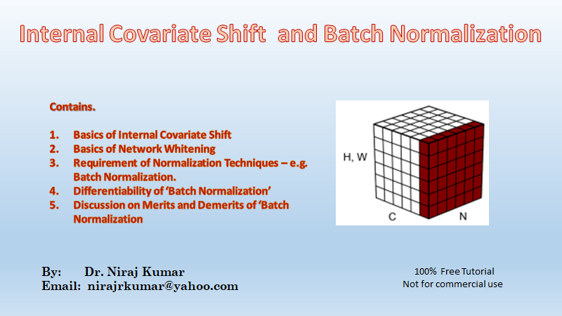
Batch Normalization Why Your Neural Network is Throwing a Tantrum (and How to Fix It)
Imagine trying to teach a toddler how to catch a ball, but every five minutes, the gravity in the room shifts, the ball changes weight, and the floor turns into a trampoline. You’d get nowhere. The toddler would get frustrated, and you’d give up.
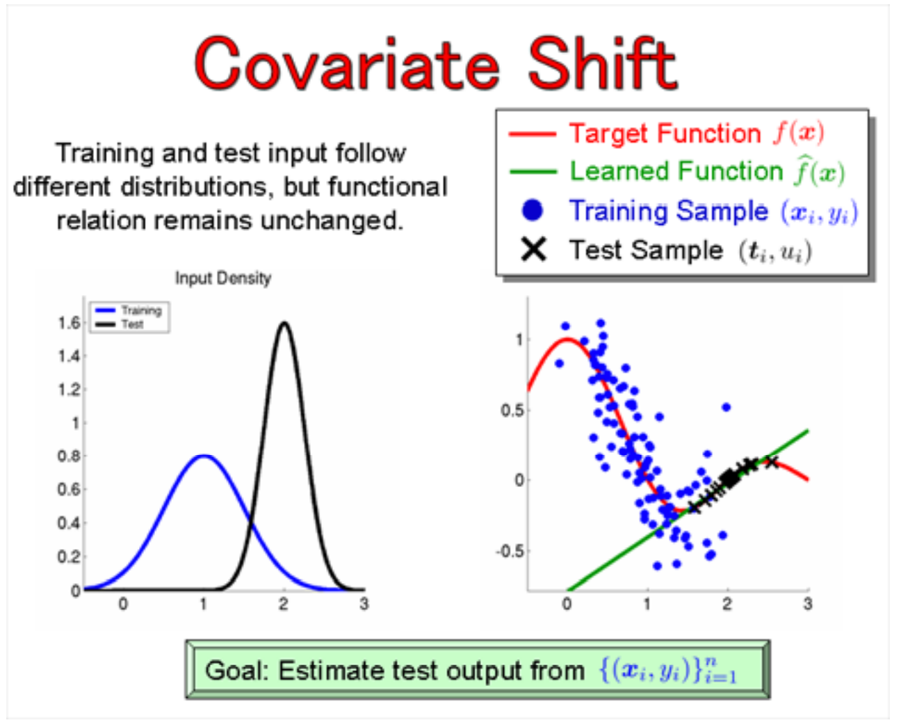
In the world of deep learning, your neural network is that toddler. As data flows through dozens of layers, the distribution of inputs to each layer changes constantly because the weights of the previous layers are updated. This phenomenon is known as Internal Covariate Shift, and it’s the reason why many models fail to converge or take forever to train.
Batch normalization is the stabilizer. It’s the hand that keeps gravity constant so your model can actually focus on learning the task at hand.
The Invisible Chaos: What is Internal Covariate Shift?
To understand why we need batch normalization, we have to look at the “hidden” struggle of a deep network. Each layer in a model is essentially a student trying to learn from the output of the layer before it.
When the first layer updates its weights, its output distribution changes. The second layer, which had just started to get comfortable with the old distribution, suddenly has to adapt to a new one. This ripple effect goes all the way down the line. It’s like trying to build a skyscraper on shifting sand; as you add more floors, the foundation keeps moving.
Batch normalization solves this by “whitening” or normalizing the inputs to each layer. It ensures that no matter how much the previous layers change, the next layer sees a distribution with a consistent mean and variance.
How Batch Normalization Actually Works (The No-Fluff Version)

Technically, batch normalization is a transformation applied to a mini-batch of data. If you’re looking for the “how-to,” the process follows four core steps for each feature:
-
Calculate the Mean: Find the average value of the mini-batch.
-
Calculate the Variance: See how spread out the data is.
-
Normalize: Subtract the mean and divide by the standard deviation. This centers the data at zero with a unit variance ($\mu = 0, \sigma = 1$).
-
Scale and Shift: This is the genius part. We introduce two learnable parameters: Gamma ($\gamma$) and Beta ($\beta$).
The “Reality Check”: Why Don’t We Just Use Standard Normalization?
A common misconception is that we want every layer to have a mean of 0 and a variance of 1. That’s actually wrong. Sometimes, a network needs a specific layer to be skewed or shifted to represent a complex feature. If we forced a hard 0/1 normalization, we might limit the model’s expressive power.
By adding $\gamma$ and $\beta$, we let the model decide: “Hey, I’ll start with normalized data, but if I think shifting it slightly to the left makes me smarter, I have the parameters to do it.”
Why You Should Care: The Practical Benefits
Implementing batch normalization isn’t just about following “best practices.” It provides tangible, bottom-line improvements to your training pipeline:
1. Faster Convergence (The Speed Demon)
Without normalization, you have to use tiny learning rates to prevent the model from exploding. With batch normalization, you can crank up the learning rate. Since the gradients are more stable, the optimizer can take much larger steps toward the “valley” of minimum loss without getting lost.
2. Resistance to Vanishing Gradients
If you’re using activation functions like Sigmoid or Tanh, you know the pain of gradients getting smaller and smaller until they disappear. By keeping the inputs in a stable range, batch normalization ensures that your activations stay in the “active” zone where gradients are healthy and informative.
3. A Hint of Regularization
Because each mini-batch is normalized using its own mean and variance, it adds a tiny bit of “noise” to the training process. Surprisingly, this acts as a slight regularizer, often reducing the need for heavy Dropout. It’s not a replacement for Dropout, but it certainly helps the model generalize better.
Where to Put It? The Architectural Debate
There’s a long-standing debate in the ML community: Do you apply batch normalization before or after the activation function?
-
The Original Paper (Ioffe & Szegedy): Recommended applying it before the activation (e.g., Linear -> BN -> ReLU).
-
Modern Practice: Many researchers have found better results applying it after the activation (e.g., Linear -> ReLU -> BN).
Editorial Opinion: While the original paper suggests “before,” there is no universal law. In modern architectures like ResNet, you’ll see variations. If your model is struggling, try swapping the order. Often, putting it after the activation leads to more stable behavior in very deep architectures.
Common Pitfalls: When Batch Normalization Fails
Despite being a “magic pill” for many, batch normalization isn’t perfect. You should be careful in these two scenarios:
-
Very Small Batch Sizes: BN relies on batch statistics. If your batch size is 2 or 4, the mean and variance will be highly inaccurate, leading to poor training. If you’re working with high-res images and tiny batches, consider Group Normalization or Layer Normalization instead.
-
Recurrent Neural Networks (RNNs): BN is notoriously tricky with sequences. Since the statistics change at every time step, applying standard BN can be messy. Layer Norm is usually the king of the castle in the RNN and Transformer world.
The Actionable Takeaway
If you are building a deep convolutional neural network today and you aren’t using batch normalization, you are essentially training with one hand tied behind your back.
Your checklist:
-
Always include BN after your Convolutional or Dense layers.
-
Start with a standard batch size (32 or 64) to give BN enough data to calculate meaningful statistics.
-
Remember to switch your model to
.eval()mode during inference so it uses the “global” moving average instead of batch statistics.
Batch normalization isn’t just a math trick; it’s the “peacekeeper” that allows deep networks to grow without collapsing under their own complexity.